Flood and chemical transport modeling

The primary physical effects to be captured that impact pollutant transport are inland flooding due to rainfall and swollen waterways, and surge inundation caused by hurricane winds. These hazard-related phenomena are further affected by tides and ocean waves. Tide levels can increase surge inundation by adding to the overall water level, while breaking waves on the coastline can add as much as 15% to surge water levels through the phenomenon of “wave set-up.” Both of these ancillary effects can modulate the severity of surge inundation.

The Delft3D model1 (also known as “Delft3D-FLOW”) used in this work was developed by Deltares, a nonprofit water research institute based in the Netherlands. Delft3D has been used in several studies in the Houston area2,3. The primary module of the model system is FLOW, a dynamic shallow water hydrodynamic model capable of simulating currents, water levels, and coastal inundation due to waves, winds, tides, and riverine flow. The model can be operated as a fully three-dimensional model or as a vertically-averaged two-dimensional model. We used the latter option, a standard choice for modeling of hurricane impacts. The model uses structured grids, and for this purpose we used a structured spherical (latitude-longitude) series of grids, with smaller, higher resolution grids receiving information from lower-resolution, larger grids, in a process known as “model nesting.”

The FLOW model requires inputs and other modules for forcing. The WAVE model, a module of Delft3D, was used to simulate the growth, propagation, and breaking of ocean surface waves. The WAVE model describes ocean waves in terms of their energy, and is a statistical representation of waves over time.

[1] Lesser, G.R., Roelvink, J.A., van Kester, J.A.T.M., and Stelling, G.S., “Development and validation of a three-dimensional morphological model.” Coastal Engineering, v 51., no. 8-9, p. 883, Oct. 2004.

[2] Zhu, R., Newman, G., Han, S., Kaihatu, J., and Wang, T., “An adaptive toolkit for projecting the impact of green infrastructure provisions on stormwater runoff and pollutant load – a case study on the city of Galena Park, Texas, USA.” Landscape Architecture Frontiers, vol. 11, no. 2, p. 72, Nov. 2023.

[3] Han, S., and Kaihatu, J.M., “Variability in surge levels in communities adjacent to the Houston Ship Channel Industrial Corridor to changes in hurricane characteristics.” Coastal Engineering Journal, doi: 10.1080/21664250.2023.22903330, Feb. 2024.

The Delft3D-FLOW model does not have a fate and transport model for industrial hazards. As a workaround, we used numerical “drogues” to track the transport of potentially-contaminated water masses in the model. These drogues are tagged numerical particles whose positions are tracked over the course of the simulation. This offers insight into the extent of contaminant transport; however, no transformation or dilution of the contaminant in flood waters is modeled.

Drogues were placed in the model at the location of facilities within each domain at the start of the simulation. The drogues remained stationary until flood waters from surge and/or riverine flooding reached them. In addition to determining the overall extent of possible contaminant transport from each facility, the drogues would also collect within topographic depressions, showing locations most at risk from contaminated floodwater.

The Delft3D-FLOW simulations comprised several domains. Winds over the entire Gulf of Mexico, and estimated tidal elevations across the Florida and Yucatan Straits, were used to generate waves and tidal elevations over the Gulf in the model. 

The overall gridded domain consisted of a series of six levels of grids, progressing toward smaller domains of higher spatial resolution. The first five levels brought waves, currents, and water levels from the Gulf of Mexico, over the Texas continental shelf and through Galveston Bay, and into the Houston Ship Channel and Buffalo Bayou region. The grid resolutions varied from 10 km for the Gulf of Mexico grid, to between 30 m to 100 m for the various gridded domains at the final grid level. The exact resolution at the final level depended on the presence of small waterways and other finescale geographic features within the domain. 

At the final level, six different subdomain grids were used to capture flooding and surge events within six different communities and immediate environs: Galena Park, Texas City, Channelview, Mont Belvieu, Laporte, and Sheldon. These six areas were selected based on the density of industry present within each, as well as flood history.

Flooding within three different time periods was simulated with the Delft3D model. During 2015, these areas experienced a relatively wet spring, while Hurricane Harvey occurred during 2017; thus these two years were simulated in the model. To represent future climate change conditions, input riverine flow from the SWAT model was increased by 7% for the time of Hurricane Harvey; the associated 2017 winds and tides were not correspondingly altered. The simulation for this climate change condition was limited to be between May 15 and October 15, rather than the entire year.

The computational time step varied depending on the spatial resolution and the CFL numerical stability criterion. For the six innermost nested spatial domains,, this time step varied between 6 seconds to 15 seconds.

Spatial maps of the water levels inside each of the six domains were output either hourly (for areas with relatively dynamic flooding) or once every two hours. Drogue positions were output at the computational time step of the simulation.

Data on the water depth (bathymetry) and land elevation (topography) were obtained from the National Center for Environmental Information (NCEI) via the Delft Dashboard model setup software. The NCEI database contains various topographical and bathymetric databases which were melded to create the terrain data for the model. For the greater Gulf of Mexico region, the General Bathymetric Chart of the Oceans (GEBCO) data set was used. This global data set is comprised of water depth data at a resolution of 15 arc-seconds (roughly 450 meters). Near to the coast, the Coastal Relief Model was used for the bathymetry and topography. This data has 1 arc-second resolution (about 30 meters). Finally, the Continuously Updated Digital Elevation Model (CUDEM) database for Texas was used where it was available. This data set has a resolution of 1/9 arc seconds (about 3 m), and was a valuable source of information for resolving the geography of creeks and waterways, as well as the Houston Ship Channel.

Winds for the year-long simulations were obtained from the Climate Forecast System Reanalysis (CFSR) database maintained by the National Center for Environmental Prediction (NCEP), NOAA. This database is comprised of a combination of modeled wind fields and satellite observations. The horizontal resolution of the data is approximately 0.5 degree latitude and longitude (about 55 km north to south and about 48 km east to west), with a one-hour temporal resolution.

For rapidly varying winds, such as those of a hurricane, the spatial resolution of the CFSR windfield may not be sufficient. This is particularly true for the Hurricane Ike case study, since the hazard for this event was primarily wind driven surge. In this event, we used the HURDAT2 database from the National Hurricane Center (NHC) for hurricane winds. This is a reduced data set which provides general parameters regarding the hurricane (radius to maximum winds, central pressure, latitude and longitude of the center along the hurricane track), as well as the distance from the center to the location of the 34 kt (17.5 m/s); 50 kt (26 m/s) and 64 kt (33 m/s) wind contours along the eight compass directions (N, S, E, W, NW, NE, SW, and SE). These are provided once every six hours, starting from when the storm is first recognized by the NHC to when the center ceases tracking it. The parameterization of Holland1 was used to fill in the wind field from these parameters.

Time series of tidal elevations were provided along the grid boundaries bisecting the Florida and Yucatan Straits, comprising the southeast corner of the Gulf of Mexico grid. The time series were provided by the Oregon State Inverse Tidal Model2, which assimilates satellite observations of sea surface height into a tidal model for accurate tidal elevations. The tidal elevations along these boundaries were then allowed to propagate into the Gulf of Mexico.

Riverine and rainfall-induced flooding were provided by the SWAT model. This input was in the form of daily-averaged discharge inflows to each of the six subdomains at locations corresponding to the boundaries of the SWAT subdomains that occur inside the six Delft3D subdomains.

All Delft3D model inputs, with the exception of CFSR winds and SWAT discharges, were accessed from the various databases by the Delft Dashboard model setup software.

[1] Holland, G., “An analytic model of the wind and pressure profiles in hurricanes.” Monthly Weather Review, v. 136, p. 1212.

[2] Egbert, G., and Erofeeva, S., “Efficient inverse modeling of barotropic ocean tides.” Journal of Atmospheric and Oceanic Technology, v. 19, p. 183, Feb. 2002

Outputs from the model consisted of wave heights, water levels, water depths, depth-averaged velocities, and other ancillary flow and wave information. These were provided at the spatial resolution of the model grid, and at a temporal resolution specified in the model input (either one or two hours). In addition, locations of drogues were also output by the model. Additional post-processing was required to make the output useful for inclusion in the vulnerability assessment as facility and community level vulnerability indicators.

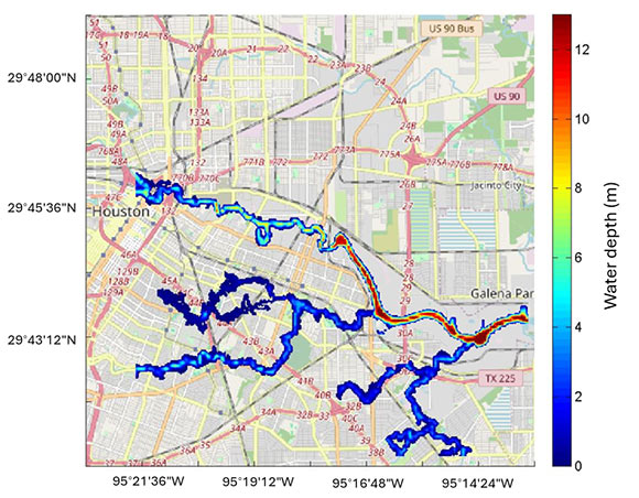
Spatial maps of water depths (water level above datum minus the local land elevation) were output by the model at the pre-set time intervals. Ensuing analysis required a metric for water depth that typified an entire year or event, so the output was analyzed to determine the maximum water depth at every grid cell over the course of a year or event. It was also necessary to eliminate cells which were filled with water under normal conditions (e.g., portions of the Ship Channel or Buffalo Bayou, rivers) from the maximum flood depth calculation. Since it requires some time for the discharge from SWAT to propagate through the Delft3D subdomain along the watercourses, each subdomain was inspected to determine the point in time when an equilibrium in water depth appeared to be reached. Areas filled with water at that time were assigned NaN (not a number) and thus eliminated as a cell for which maximum flood elevation was calculated.

Another important flood characterization parameter is residence time – the length of time that flood water remains in an area. Since it is difficult for the model to go to zero water depth after flooding, we instead looked at the slope of the water depth with time. A positive slope (increasing water depth) indicates that the area is filling with water, while a negative slope (decreasing water depth) denotes drainage out of the area. For any given cell, we tracked the time from the point where the water depth slope over time went from positive, to the point where a negative slope was quickly followed by a slightly positive slope or a zero slope. The difference between those times was used as the residence time for that specific flooding event in that grid cell, which may have been one of several over the course of a year. The maximum, minimum, and average retention time over the course of a year or event was then determined for each cell.

Drogues were placed in the model at the locations of facilities, at the beginning of the simulation. These locations are always dry until reached by flood waters. The specific scenario replicated would be the case of a spill occurring prior to flooding, with flood water then transporting the spilled material through the domain.

Most information from the model and used in the vulnerability assessment and other tools were processed using MATLAB codes developed within the project. Translation between the native NEutral FIle System (NEFIS) format (developed by Deltares) and MATLAB binary formats was performed using MATLAB routines developed by Deltares. In-house MATLAB codes were then developed to perform the required analyses from the model results. Maps of residence time and maximum flood depths were output in TIFF format. Drogue tracks were written into ASCII files identified by facility ID. Each drogue file consisted of three columns: time (in minutes) from the start time of the simulation, and latitude and longitude of the drogue.